Minimization of nonlinear energy functional

In this example we solve the following nonlinear minimization problem

Find $u^* \in H^1_0(\Omega)$ such that

Here the energy functional $\Pi(u)$ has the form

where

Necessary optimality condition (Euler-Lagrange condition)

Let $\delta_u \Pi(u, \hat{u})$ denote the first variation of $\Pi(u)$ in the direction $\hat{u}$, i.e.

The necessary condition is that the first variation of $\Pi(u)$ equals to 0 for all directions $\hat{u}$:

Weak form:

To obtain the weak form of the above necessary condition, we first expand the term $\Pi(u + \varepsilon \hat{u})$ as

After some simplification, we obtain

By neglecting the $\mathcal{O}(\epsilon)$ terms, we write the weak form of the necessary conditions as

Find $u\in H_0^1(\Omega)$ such that

Strong form:

To obtain the strong form, we invoke Green’s first identity and write

Since $\hat{u}$ is arbitrary in $\Omega$ and $\hat{u} = 0$ on $\partial \Omega$, the strong form of the non-linear boundary problem reads

$- \nabla \cdot [(k_1 + k_2u^2) \nabla u + k_2 u \nabla u \cdot \nabla u = f \quad {\rm in} \; \Omega;$ $u = 0 \quad {\rm on} \; \partial\Omega.$

Infinite-dimensional Newton’s Method

Consider the expansion of the first variation $\delta_u \Pi(u, \hat{u})$ about $u$ in a direction $\tilde{u}$

where

The infinite-dimensional Newton’s method reads

Given the current solution $u_k$, find $\tilde{u} \in H^1_0$ such that

Update the solution using the Newton direction $\tilde{u}$ $u_{k+1} = u_k + \tilde{u}.$

Hessian

To derive the weak form of the Hessian, we first expand the term $\delta_u \Pi(u +\varepsilon \tilde{u},\hat{u})$ as

Then, after some simplification, we obtain

Weak form of Newton step:

Given $u \in H_0^1$, find $\tilde{u} \in H^1_0$ such that

The solution is then updated using the Newton direction $\tilde{u}$

Here $\alpha$ denotes a relaxation parameter (back-tracking/line-search) used to achieve global convergence of the Newton method.

Strong form of the Newton step

$- \nabla \cdot \left[ (k_1 + k_2 u^2) \nabla \tilde{u}\right] + 2k_2u\nabla\tilde{u}\cdot\nabla u - \nabla\cdot(2k_2 u \tilde{u} \nabla u) + k_2 \tilde{u} \nabla u \nabla u = \nabla \cdot\left[(k_1 + k_2 u^2)\nabla \right]u - k_2 u \nabla u\cdot \nabla u + f \quad {\rm in} \, \Omega.$ $\tilde{u} = 0 \quad {\rm on} \, \partial \Omega.$

1. Load modules

To start we load the following modules:

• dolfin: the python/C++ interface to FEniCS

• math: the python module for mathematical functions

• numpy: a python package for linear algebra

• matplotlib: a python package used for plotting the results

from __future__ import print_function, division, absolute_import

import dolfin as dl

import matplotlib.pyplot as plt
%matplotlib inline

from hippylib import nb

import math
import numpy as np
import logging

logging.getLogger('FFC').setLevel(logging.WARNING)
logging.getLogger('UFL').setLevel(logging.WARNING)
dl.set_log_active(False)

2. Define the mesh and finite element spaces

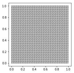
We construct a triangulation (mesh) $\mathcal{T}_h$ of the computational domain $\Omega := [0, 1]^2$ with nx elements in the x-axis direction and ny elements in the y-axis direction.

On the mesh $\mathcal{T}_h$, we then define the finite element space $V_h \subset H^1(\Omega)$ consisting of globally continuous piecewise linear functions and we create a function $u \in V_h$.

By denoting by $\left[{\phi_i(x)}\right]_{i=1}^{ {\rm dim}(V_h)}$ the finite element basis for the space $V_h$ we have $u = \sum_{i=1}^{ {\rm dim}(V_h)} {\rm u}_i \phi_i(x),$ where ${\rm u}_i$ represents the coefficients in the finite element expansion of $u$.

Finally we define two special types of functions: the TestFunction $\hat{u}$ and the TrialFunction $\tilde{u}$. These special types of functions are used by FEniCS to generate the finite element vectors and matrices which stem from the first and second variations of the energy functional $\Pi$.

nx = 32
ny = 32
mesh = dl.UnitSquareMesh(nx,ny)
Vh = dl.FunctionSpace(mesh, "CG", 1)

uh = dl.Function(Vh)
u_hat = dl.TestFunction(Vh)
u_tilde = dl.TrialFunction(Vh)

nb.plot(mesh, show_axis="on")
print( "dim(Vh) = ", Vh.dim() )

dim(Vh) =  1089

3. Define the energy functional

We now define the energy functional $\Pi(u) = \frac{1}{2} \int_\Omega (k_1 + k_2u^2) \nabla u \cdot \nabla u dx - \int_\Omega f\,u dx.$

The parameters $k_1$, $k_2$ and the forcing term $f$ are defined in FEniCS using the keyword Constant. To define coefficients that are space dependent one should use the keyword Expression.

The Dirichlet boundary condition $u = 0 \quad {\rm on} \; \partial\Omega$ is imposed using the DirichletBC class.

To construct this object we need to provide

• the finite element space Vh

• the value u_0 of the solution at the Dirichlet boundary. u_0 can either be a Constant or an Expression object.

• the object Boundary that defines on which part of $\partial \Omega$ we want to impose such condition.

f = dl.Constant(1.)
k1 = dl.Constant(0.05)
k2 = dl.Constant(1.)

Pi = dl.Constant(.5)*(k1 + k2*uh*uh)*dl.inner(dl.grad(uh), dl.grad(uh))*dl.dx - f*uh*dl.dx

class Boundary(dl.SubDomain):
    def inside(self, x, on_boundary):
        return on_boundary

u_0 = dl.Constant(0.)    
bc = dl.DirichletBC(Vh,u_0, Boundary() )

4. First variation

The weak form of the first variation reads

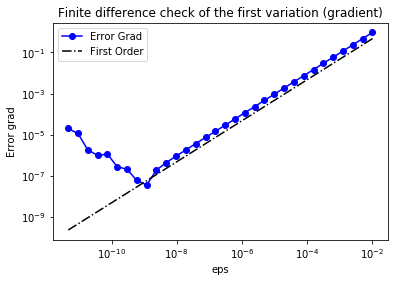
We use a finite difference check to verify that our derivation is correct. More specifically, we consider a function $u_0 = x(x-1)y(y-1) \in H^1_0(\Omega)$ and we verify that for a random direction $\hat{u} \in H^1_0(\Omega)$ we have $r := \left| \frac{\Pi(u_0 + \varepsilon \hat{u}) - \Pi(u_0)}{\varepsilon} - \delta_u \Pi(u, \hat{u})\right| = \mathcal{O}(\varepsilon).$

In the figure below we show in a loglog scale the value of $r$ as a function of $\varepsilon$. We observe that $r$ decays linearly for a wide range of values of $\varepsilon$, however we notice an increase in the error for extremely small values of $\varepsilon$ due to numerical stability and finite precision arithmetic.

NOTE: To compute the first variation we can also use the automatic differentiation of variational forms capabilities of FEniCS and write

grad = dl.derivative(Pi, u, u_hat)

grad = (k2*uh*u_hat)*dl.inner(dl.grad(uh), dl.grad(uh))*dl.dx + \
       (k1 + k2*uh*uh)*dl.inner(dl.grad(uh), dl.grad(u_hat))*dl.dx - f*u_hat*dl.dx

u0 = dl.interpolate(dl.Expression("x[0]*(x[0]-1)*x[1]*(x[1]-1)", degree=2), Vh)

n_eps = 32
eps = 1e-2*np.power(2., -np.arange(n_eps))
err_grad = np.zeros(n_eps)

uh.assign(u0)
pi0 = dl.assemble(Pi)
grad0 = dl.assemble(grad)

uhat = dl.Function(Vh).vector()
uhat.set_local(np.random.randn(Vh.dim()))
uhat.apply("")
bc.apply(uhat)
dir_grad0 = grad0.inner(uhat)

for i in range(n_eps):
    uh.assign(u0)
    uh.vector().axpy(eps[i], uhat) #uh = uh + eps[i]*dir
    piplus = dl.assemble(Pi)
    err_grad[i] = abs( (piplus - pi0)/eps[i] - dir_grad0 )

plt.figure()    
plt.loglog(eps, err_grad, "-ob", label="Error Grad")
plt.loglog(eps, (.5*err_grad[0]/eps[0])*eps, "-.k", label="First Order")
plt.title("Finite difference check of the first variation (gradient)")
plt.xlabel("eps")
plt.ylabel("Error grad")
plt.legend(loc = "upper left")
plt.show()

5. Second variation

The weak form of the second variation reads

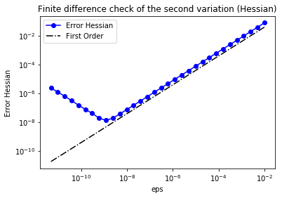
As before, we verify that for a random direction $\hat{u} \in H^1_0(\Omega)$ we have $r := \left\| \frac{\delta_u\Pi(u_0 + \varepsilon \tilde{u}, \hat{u}) - \delta_u \Pi(u_0, \hat{u})}{\varepsilon} - \delta_u^2 \Pi(u, \tilde{u}, \hat{u})\right\| = \mathcal{O}(\varepsilon).$

In the figure below we show in a loglog scale the value of $r$ as a function of $\varepsilon$. As before, we observe that $r$ decays linearly for a wide range of values of $\varepsilon$, however we notice an increase in the error for extremely small values of $\varepsilon$ due to numerical stability and finite precision arithmetic.

NOTE: To compute the second variation we can also use automatic differentiation and write

H = dl.derivative(grad, u, u_tilde)

H = k2*u_tilde*u_hat*dl.inner(dl.grad(uh), dl.grad(uh))*dl.dx + \
     dl.Constant(2.)*(k2*uh*u_hat)*dl.inner(dl.grad(u_tilde), dl.grad(uh))*dl.dx + \
     dl.Constant(2.)*k2*u_tilde*uh*dl.inner(dl.grad(uh), dl.grad(u_hat))*dl.dx + \
     (k1 + k2*uh*uh)*dl.inner(dl.grad(u_tilde), dl.grad(u_hat))*dl.dx

uh.assign(u0)
H_0 = dl.assemble(H)
H_0uhat = H_0 * uhat
err_H = np.zeros(n_eps)

for i in range(n_eps):
    uh.assign(u0)
    uh.vector().axpy(eps[i], uhat)
    grad_plus = dl.assemble(grad)
    diff_grad = (grad_plus - grad0)
    diff_grad *= 1/eps[i]
    err_H[i] = (diff_grad - H_0uhat).norm("l2")
    
plt.figure()    
plt.loglog(eps, err_H, "-ob", label="Error Hessian")
plt.loglog(eps, (.5*err_H[0]/eps[0])*eps, "-.k", label="First Order")
plt.title("Finite difference check of the second variation (Hessian)")
plt.xlabel("eps")
plt.ylabel("Error Hessian")
plt.legend(loc = "upper left")
plt.show()

6. The infinite dimensional Newton Method

The infinite dimensional Newton step reads

Given $u_n \in H_0^1$, find $\tilde{u} \in H^1_0$ such that

Update the solution $u_{n+1}$ using the Newton direction $\tilde{u}$

Here, for simplicity, we choose $\alpha$ equal to 1. In general, to guarantee global convergence of the Newton method the parameter $\alpha$ should be appropriately chosen (e.g. back-tracking or line search).

The linear systems to compute the Newton directions are solved using the conjugate gradient (CG) with algebraic multigrid preconditioner with a fixed tolerance. In practice, one should solve the Newton system inexactly by early termination of CG iterations via Eisenstat–Walker (to prevent oversolving) and Steihaug (to avoid negative curvature) criteria.

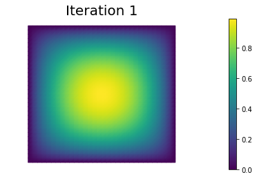
In the output below, for each iteration we report the number of CG iterations, the value of the energy functional, the norm of the gradient, and the inner product between the gradient and the Newton direction $\delta_u \Pi(u_0, \tilde{u})$.

In the example, the stopping criterion is relative norm of the gradient $\frac{\delta_u \Pi(u_n, \hat{u})}{\delta_u \Pi(u_0, \hat{u})} \leq \tau$. However robust implementation of the stopping criterion should monitor also the quantity $\delta_u \Pi(u_0, \tilde{u})$.

uh.assign(dl.interpolate(dl.Constant(0.), Vh))

rtol = 1e-9
max_iter = 10

pi0 = dl.assemble(Pi)
g0 = dl.assemble(grad)
bc.apply(g0)
tol = g0.norm("l2")*rtol

du = dl.Function(Vh).vector()

lin_it = 0
print ("{0:3} {1:3} {2:15} {3:15} {4:15}".format(
      "It", "cg_it", "Energy", "(g,du)", "||g||l2") )

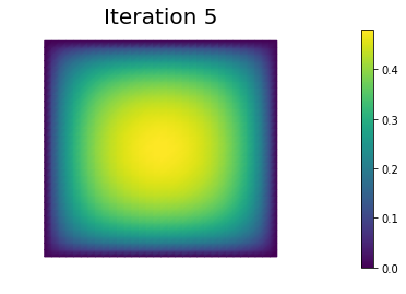
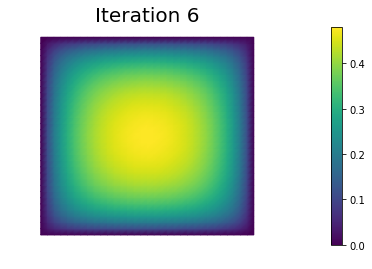
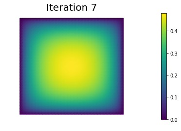
for i in range(max_iter):
    [Hn, gn] = dl.assemble_system(H, grad, bc)
    if gn.norm("l2") < tol:
        print ("\nConverged in ", i, "Newton iterations and ", lin_it, "linear iterations.")
        break
    myit = dl.solve(Hn, du, gn, "cg", "petsc_amg")
    lin_it = lin_it + myit
    uh.vector().axpy(-1., du)
    pi = dl.assemble(Pi)
    print ("{0:3d} {1:3d} {2:15e} {3:15e} {4:15e}".format(
      i, myit, pi, -gn.inner(du), gn.norm("l2")) )
    
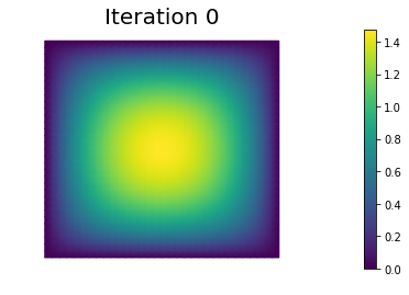
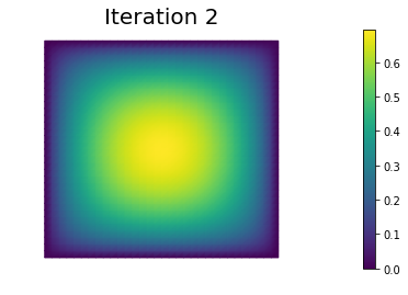
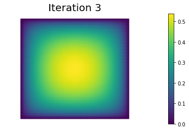
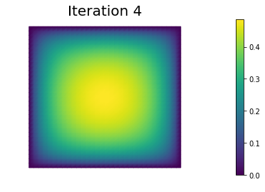
    plt.figure()
    nb.plot(uh, mytitle="Iteration {0:1d}".format(i))
    
plt.show()

It  cg_it Energy          (g,du)          ||g||l2        
  0   4    2.131680e+00   -7.006604e-01    3.027344e-02
  1   3    1.970935e-01   -3.236483e+00    4.776453e-01
  2   3   -1.353236e-01   -5.650329e-01    1.383328e-01
  3   3   -1.773194e-01   -7.431340e-02    3.724056e-02
  4   4   -1.796716e-01   -4.455251e-03    7.765301e-03
  5   4   -1.796910e-01   -3.850049e-05    7.391677e-04
  6   4   -1.796910e-01   -4.633942e-09    9.309628e-06
  7   4   -1.796910e-01   -8.692570e-17    1.501038e-09

Converged in  8 Newton iterations and  29 linear iterations.

uh.assign(dl.interpolate(dl.Constant(0.), Vh))
parameters={"symmetric": True, "newton_solver": {"relative_tolerance": 1e-9, "report": True, \
                                                 "linear_solver": "cg", "preconditioner": "petsc_amg"}}
dl.solve(grad == 0, uh, bc, J=H, solver_parameters=parameters)
final_g = dl.assemble(grad)
bc.apply(final_g)

print ( "Norm of the gradient at converge", final_g.norm("l2") )
print ("Value of the energy functional at convergence", dl.assemble(Pi) )
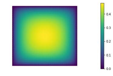
nb.plot(uh)
plt.show()

Norm of the gradient at converge 8.041168028721095e-15
Value of the energy functional at convergence -0.17969096618442762

Hands on

Consider the following nonlinear minimization problem

Find $u^* \in H^1(\Omega)$ such that

where

Question 1

Derive the first-order necessary condition for optimality using calculus of variations, in both weak and strong form.

Let $\delta_u \Pi(u, \hat{u})$ denote the first variation of $\Pi(u)$ in the direction $\hat{u}$, i.e.

The necessary condition is that the first variation of $\Pi(u)$ equals to 0 for all directions $\hat{u}$:

To obtain the weak form of the above necessary condition, we first expand the term $\Pi(u + \varepsilon \hat{u})$ as

Then, we have

After setting $\varepsilon = 0$, we write the weak form of the necessary conditions as

Find $u\in H^1(\Omega)$ such that

To obtain the strong form, we invoke Green’s first identity and write

Since $\hat{u}$ is arbitrary in $\Omega$ and on $\partial \Omega$, the strong form of the non-linear boundary problem reads

$- \Delta u - e^{-u} = 0 \quad {\rm in} \; \Omega;$ $\nabla u \cdot \boldsymbol{n} + u = 0 \quad {\rm on} \; \partial\Omega.$

Note: The boundary condition $\nabla u \cdot \boldsymbol{n} + u = 0$ is a Robin type boundary condition.

Question 2

Derive the infinite-dimensional Newton step, in both weak and strong form.

To derive the infinite-dimensional Newton step, we first compute the second variation of $\Pi$, that is

After some simplification, we obtain

The weak form of Newton step then reads

Given $u^{(n)} \in H^1$, find $\tilde{u} \in H^1$ such that

Update the solution using the direction $\tilde{u}$

Here $\alpha$ denotes a relaxation parameter (back-tracking/line-search) used to achieve global convergence of the Newton method.

Finally the strong form of the Newton step reads

$- \Delta \tilde{u} + e^{-u^{(n)}}\tilde{u} = \Delta u^{(n)} + e^{-u^{(n)}} \quad {\rm in} \; \Omega;$ $\nabla \tilde{u} \cdot \boldsymbol{n} + \tilde{u}= -\nabla u^{(n)} \cdot \boldsymbol{n} - u^{(n)} \quad {\rm on} \; \partial\Omega.$

Question 3

Discretize and solve the above nonlinear minimization problem using FEniCS.

nx = 32
ny = 32
mesh = dl.UnitSquareMesh(nx,ny)
Vh = dl.FunctionSpace(mesh, "CG", 1)

uh = dl.Function(Vh)
u_hat = dl.TestFunction(Vh)
u_tilde = dl.TrialFunction(Vh)

print( "dim(Vh) = ", Vh.dim() )

Pi   = dl.Constant(.5)*dl.inner(dl.grad(uh), dl.grad(uh))*dl.dx + dl.exp(-uh)*dl.dx + dl.Constant(.5)*uh*uh*dl.ds
grad = dl.inner(dl.grad(u_hat), dl.grad(uh))*dl.dx - u_hat*dl.exp(-uh)*dl.dx + uh*u_hat*dl.ds
H    = dl.inner(dl.grad(u_hat), dl.grad(u_tilde))*dl.dx + u_hat*u_tilde*dl.exp(-uh)*dl.dx + u_tilde*u_hat*dl.ds

uh.assign(dl.interpolate(dl.Constant(0.), Vh))

rtol = 1e-9
max_iter = 10

pi0 = dl.assemble(Pi)
g0 = dl.assemble(grad)
tol = g0.norm("l2")*rtol

du = dl.Function(Vh).vector()

lin_it = 0
print ("{0:3} {1:3} {2:15} {3:15} {4:15}".format(
      "It", "cg_it", "Energy", "(g,du)", "||g||l2") )

for i in range(max_iter):
    [Hn, gn] = dl.assemble_system(H, grad)
    if gn.norm("l2") < tol:
        print ("\nConverged in ", i, "Newton iterations and ", lin_it, "linear iterations.")
        break
    myit = dl.solve(Hn, du, gn, "cg", "petsc_amg")
    lin_it = lin_it + myit
    uh.vector().axpy(-1., du)
    pi = dl.assemble(Pi)
    print ("{0:3d} {1:3d} {2:15e} {3:15e} {4:15e}".format(
      i, myit, pi, -gn.inner(du), gn.norm("l2")) )
      
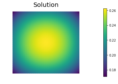
plt.figure()
nb.plot(uh, mytitle="Solution", )
plt.show()

dim(Vh) =  1089
It  cg_it Energy          (g,du)          ||g||l2        
  0   4    8.858149e-01   -2.247173e-01    3.076215e-02
  1   4    8.857473e-01   -1.352648e-04    7.406045e-04
  2   5    8.857473e-01   -3.976430e-11    5.593599e-07
  3   6    8.857473e-01   -1.214857e-21    4.624314e-11

Converged in  4 Newton iterations and  19 linear iterations.

Copyright © 2016-2018, The University of Texas at Austin & University of California, Merced.
All Rights reserved.
See file COPYRIGHT for details.

This file is part of the hIPPYlib library. For more information and source code availability see https://hippylib.github.io.

hIPPYlib is free software; you can redistribute it and/or modify it under the terms of the GNU General Public License (as published by the Free Software Foundation) version 2.0 dated June 1991.