Introduction to Sampling Methods

Goals

There are two goals for this lab:

To further acquaint you with MUQ, including random number generators and model construction.
To develop a deeper understanding of methods for sampling from general distributions
- Nonlinear transformations
- Rejection Sampling
- Markov chain Monte Carlo (MCMC)
- Importance Sampling

Problem Description

To illustrate these topics, we will consider the infamous “Banana” distribution, which is also called the “Boomerang” distribution in some circles.

Consider a standard normal random variable $z\sim N(0,I)$. For some $a,b>0$, consider the transformation $m=S(z)$ given by

$m = \left[\begin{array}{c} m_1 \\ m_2 \end{array} \right] = S(z) = \left[\begin{array}{l} a z_1 \\ \frac{1}{a} z_2 + b (az_1)^2 + ba^2 \end{array}\right].$

With this transformation, sampling $m$ can be accomplished by drawing a random sample of $z$ and then evaluating $S(z)$.

We will also sample $m$ using other methods that require evaluating the density $p(m)$. To evaluate the density, we need to inverse transformation $T(m)=z$, which takes the form

$z = \left[\begin{array}{c} z_1 \\ z_2 \end{array} \right] = T(m) = \left[\begin{array}{l} \frac{1}{a} m_1 \\ a m_2 + ab(m_1^2 + a^2) \end{array}\right].$

Let $p_z(z)$ denote the Gaussian density on $z$. Then the density on $M$ is given by

$p_m(m) = p_z(T(m))\,\left|\det{\nabla T}\right|$

where $\left\vert\det{\nabla T}\right\vert$ denotes the determinant of the Jacobian matrix of $T(m)$ . The $p_m(m)$ is the banana density and (for $a=1$) it looks like:

The form of $p_m(m)$ can also be simplified by considering the determinant term in more detail. The Jacobian is given by

$\nabla T(m) = \left[ \begin{array}{cc} \frac{1}{a} & 0\\ 2ab m_1& a\end{array} \right].$

The determinant of a lower triangular matrix is the product of the digaonal entries, so $\left\vert\det{\nabla T}\right\vert = \frac{1}{a} a$. Interestingly, the determinant of this Jacobian is always $1$, regardless of $a$ and $m$! Thus, for this problem $p_m(m) = p_z(T(m))$. It is important to note that this is a very special case and in general, the determinant term is required to define $p_m(m)$.

import sys
sys.path.insert(0,'/home/fenics/Installations/MUQ_INSTALL/lib')

import matplotlib.pyplot as plt
import matplotlib.cm as cm
import numpy as np

from IPython.display import Image

import pymuqUtilities as mu
from pymuqUtilities import RandomGenerator as rg

import pymuqModeling as mm

Background: Simple Random number generation

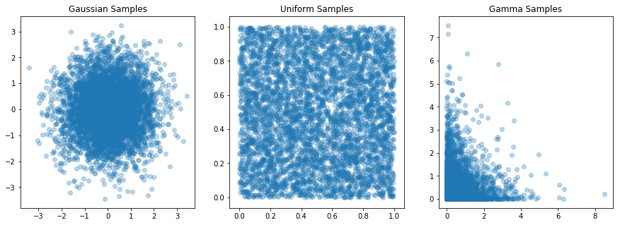
Below are a few examples of generating random variables in MUQ for a few canonical distributions. The functions described here will serve as building blocks for more sophisticated sampling techniques.

Continuous Random Variables

numSamps = 5000
paramDim = 2

rg.SetSeed(2012)

# Gaussian Samples
gaussScalar = rg.GetNormal()
gaussVector = rg.GetNormal(paramDim)
gaussMatrix = rg.GetNormal(paramDim, numSamps)

# Uniform Samples
uniformScalar = rg.GetUniform()
uniformVector = rg.GetUniform(paramDim)
uniformMatrix = rg.GetUniform(paramDim, numSamps)

# Gamma Samples
gammaAlpha = 0.5
gammaBeta = 1.0

gammaScalar = rg.GetGamma(gammaAlpha, gammaBeta)
gammaVector = rg.GetGamma(gammaAlpha, gammaBeta, paramDim)
gammaMatrix = rg.GetGamma(gammaAlpha, gammaBeta, paramDim, numSamps)

fig, axs = plt.subplots(ncols=3, figsize=(15,5))
axs[0].scatter(gaussMatrix[0,:], gaussMatrix[1,:], alpha=0.3)
axs[0].set_title('Gaussian Samples')

axs[1].scatter(uniformMatrix[0,:], uniformMatrix[1,:], alpha=0.3)
axs[1].set_title('Uniform Samples')

axs[2].scatter(gammaMatrix[0,:], gammaMatrix[1,:], alpha=0.3)
axs[2].set_title('Gamma Samples')


plt.show()

png

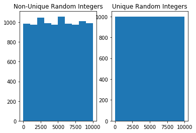
Integer Random Variables

lb = 0
ub = paramDim*numSamps

isUnique = False
intScalar = rg.GetUniformInt(lb,ub)
intVector = rg.GetUniformInt(lb, ub, paramDim, isUnique)
intMatrix = rg.GetUniformInt(lb, ub, paramDim, numSamps, isUnique)

isUnique = True
uniqueIntScalar = rg.GetUniformInt(lb, ub)
uniqueIntVector = rg.GetUniformInt(lb, ub, paramDim, isUnique)
uniqueIntMatrix = rg.GetUniformInt(lb, ub, paramDim, numSamps, isUnique)

fig, axs = plt.subplots(ncols=2)

axs[0].hist(intMatrix.ravel())
axs[0].set_title('Non-Unique Random Integers')

axs[1].hist(uniqueIntMatrix.ravel())
axs[1].set_title('Unique Random Integers')

Text(0.5,1,'Unique Random Integers')

png

The MUQ `ModPiece` class

MUQ provides many tools that need to interact with user defined models or model components. The MUQ ModPiece class provides a mechanism for defining models (i.e., input-output relationships) in a way that MUQ can understand. To define a new model, the user creates a class that inherits from the PyModPiece class (or just ModPiece in c++), overrides the EvaluateImpl function, and tells the parent PyModPiece class the size and number of inputs and outputs the new model has. Note that these model components can have multiple inputs and multiple outputs.

For more information on classes and inheritance in Python, check out this introduction.

For example, the following class implements the “Banana” transformation from $z\rightarrow m$.

The EvaluateImpl function takes a list of input vectors and sets the self.outputs member variable, which is also a list of vectors.

The __init__ function in the BananaTrans class must call PyModPiece.__init__ and specify the number of inputs and outputs. The PyModPiece.__init__ function has three inputs:

self
A list of integers specifying the size of each model input
A list of integers specifying the size of each model output

class BananaTrans(mm.PyModPiece):
    def __init__(self, a, b):
        mm.PyModPiece.__init__(self, [2], # One input containing 2 components
                                     [2]) # One output containing 2 components
        
        self.a = a
        self.b = b
        
    def EvaluateImpl(self, inputs):
        z = inputs[0]
        
        m = np.zeros((2))
        m[0] = self.a * z[0]
        m[1] = z[1]/self.a - self.b*((self.a*z[0])**2 + self.a**2)
        
        self.outputs = [m]

        

Derivatives in the `ModPiece` class

Many algorithms require derivative information to be efficient. To add this information to a child of PyModPiece, we can override additional functions. In particular,

the JacobianImpl function can be overridden to implement the Jacobian
the GradientImpl function can be overriden to implement Gradients, including adjoint gradients (i.e., computation of $J^Tv$ for some vector $v$)
the ApplyJacobianImpl function can be overriden to implement Jacobian actions (i.e., $Jv$)

Below, we override the JacobianImpl function in the inverse banana transformation to provide Jacobian information.

class InvBananaTrans(mm.PyModPiece):
    
    def __init__(self, a, b):
        mm.PyModPiece.__init__(self, [2], # One input containing 2 components
                                     [2]) # One output containing 2 components
        self.a = a
        self.b = b
        print(self.a)
        
    def EvaluateImpl(self, inputs):
        m = inputs[0]
        
        z = np.zeros((2))
        z[0] = m[0]/self.a
        z[1] = m[1]*self.a + self.a*self.b*(m[0]**2 + self.a**2)
        self.outputs = [z]
        
    def JacobianImpl(self, outDimWrt, inDimWrt, inputs):
        m = inputs[0]
        self.jacobian = np.array([ [1.0/self.a, 0], [2.0*self.a*self.b*m[0], self.a] ])
        
    # TODO: Override the GradientImpl function, i.e. $J^T v$, where $v$ is the "sens" input
    def GradientImpl(self, outDimWrt, inDimWrt, inputs, sens):
    #     ...  Do a bunch of stuff here ...
    #     self.gradient = ?     
        self.gradient = self.Jacobian(outDimWrt, inDimWrt, inputs).T @ sens

a = 1.0
b = 1.0
invf = InvBananaTrans(a,b)

# TODO: Test your gradient by comparing it with a finite difference gradient
sens = np.ones((2))
m = np.array([0,-2])

fdGrad = invf.GradientByFD(0,0,[m],sens)
grad = invf.Gradient(0,0,[m],sens)

print('Finite Difference Gradient =\n', fdGrad)
print('Analytical Gradient =\n', grad)

1.0
Finite Difference Gradient =
 [ 1.          0.99999999]
Analytical Gradient =
 [ 1.  1.]

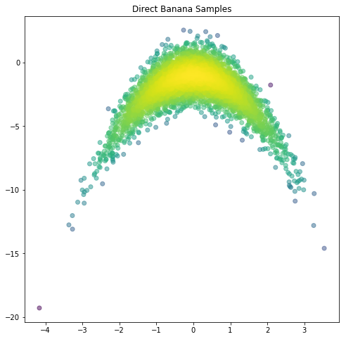
Sampling via Nonlinear Transformations

# Illustration that ModPiece output is a list
f = BananaTrans(a,b)

z = np.array([0,0])
modPieceOutput = f.Evaluate([ z ])

print('Transformation Output = \n', modPieceOutput)

Transformation Output = 
 [array([ 0., -1.])]

zDist = mm.Gaussian(np.zeros((paramDim)))

# TODO: Use the f object to generate "numSamps" samples of the banana random variable m
# RECALL: The Gaussian class has a Sample() function

mSamps = np.zeros((paramDim, numSamps))
for i in range(numSamps):
    mSamps[:,i] = f.Evaluate([ zDist.Sample() ])[0]
    

# TODO: For each sample above, use the invf compute the value of the banana density
# RECALL: The Gaussian distribution from Friday has a LogDensity(z) function

logDensVals1 = np.zeros(numSamps)

for i in range(numSamps):
    jac = invf.Jacobian(0,0, [ mSamps[:,i] ])
    z = invf.Evaluate([ mSamps[:,i] ])
    logDensVals1[i] = zDist.LogDensity(z) + np.linalg.slogdet(jac)[1]

# TODO: Create a scatter plot of the banana samples (hint: use plt.scatter)

plt.figure(figsize=(8,8))

plt.scatter(mSamps[0,:],mSamps[1,:],c=logDensVals1, alpha=0.5)
plt.title('Direct Banana Samples')
plt.show()

png

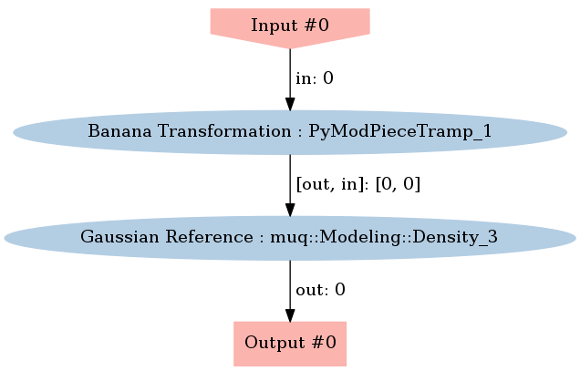
The WorkGraph class

In MUQ, the WorkGraph class allows us to combine multiple model components (i.e., ModPiece instance). Here, we will create a new model that evaluates $\log p_m(m) = \log p_z(T(m))$. We will do this by combining an instance of InvBananaTrans with a Gaussian density.

First, we need to construct a graph with two nodes and one edge.

graph = mm.WorkGraph()

graph.AddNode(zDist.AsDensity(), "Gaussian Reference")
graph.AddNode(invf, "Banana Transformation")

graph.AddEdge("Banana Transformation", 0, "Gaussian Reference", 0)

graph.Visualize("EvaluationGraph.png")
Image(filename='EvaluationGraph.png') 

png

Now that the graph is constructed, we can create the new model (in the form of a ModPiece). Here, we use the CreateModPiece function, but takes the name of the output node as an argument.

tgtDens = graph.CreateModPiece("Gaussian Reference")

# TODO: Use the tgtDens.Evaluate function to evaluate $\log p_m(m)$ at each sample point.

logDensVals2 = np.zeros(numSamps)

for i in range(numSamps):
    logDensVals2[i] = tgtDens.Evaluate([ mSamps[:,i] ])[0] # NOTE: This only works because the jacobian is 1

# TODO: Plot the new density evaluations, do they match the results above?

plt.figure(figsize=(8,8))

plt.scatter(mSamps[0,:],mSamps[1,:],c=logDensVals2, alpha=0.5)
plt.title('Direct Banana Samples')
plt.show()

png

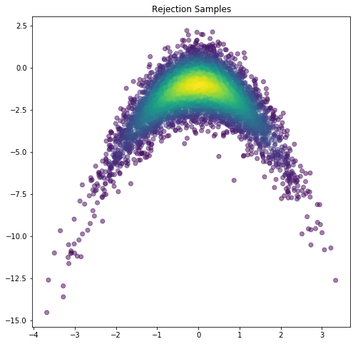
Rejection Sampling

propMu = np.array([0,-4])
propCov = np.array([ [4, 0],
                     [0, 20]])

propDist = mm.Gaussian(propMu, propCov)

rejectSamps = np.zeros((paramDim, numSamps))
rejectDens = np.zeros((numSamps))

# TODO: Implement a rejection sampler that samples from the banana density.

numAccepts = 0
numProposed = 0
M = np.exp(3)

while(numAccepts < numSamps):
    numProposed += 1
    
    # Propose in the banana space
    mprop = propDist.Sample()
    
    # Evaluate the log target density
    logTgt = tgtDens.Evaluate([ mprop ])[0]
    
    # Evaluate the log proposal density
    logProp = propDist.LogDensity(mprop)
    
    # Compute the acceptance ratio
    alpha = np.exp(logTgt - np.log(M) - logProp)
    
    assert logTgt < np.log(M) + logProp
    
    # Accept with probability alpha
    if(rg.GetUniform() < alpha):
        rejectSamps[:,numAccepts] = mprop
        rejectDens[numAccepts] = logTgt
        numAccepts += 1
        
print('%d target density evaluations were needed to compute %d samples'%(numProposed, numSamps))

99350 target density evaluations were needed to compute 5000 samples

plt.figure(figsize=(8,8))

plt.scatter(rejectSamps[0,:], rejectSamps[1,:], c=np.exp(rejectDens), alpha=0.5)
plt.title('Rejection Samples')
plt.show()

png

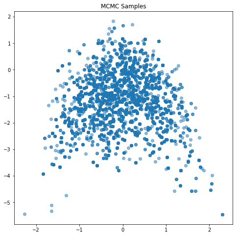
Markov Chain Monte Carlo Sampling

propMu = np.zeros((paramDim))
propCov = 4.0*np.eye(paramDim)

mcmcProp = mm.Gaussian(propMu, propCov)

mcmcSamps = np.zeros((paramDim, numSamps))
mcmcDens = np.zeros((numSamps))

# TODO: Implement a simple random walk Metropolis algorithm to sample from the banana density.

currPt = np.zeros((paramDim))
currLogTgt = tgtDens.Evaluate([currPt])[0]

numAccepts = 0

for i in range(numSamps):
    propSamp = mcmcProp.Sample()
    
    propLogTgt = tgtDens.Evaluate([propSamp])[0]
    
    u = np.exp(propLogTgt - currLogTgt)
    if(rg.GetUniform() < u):
        numAccepts += 1
        
        mcmcSamps[:,i] = propSamp
        
        currPt = propSamp
        currLogTgt = propLogTgt
    else:
        mcmcSamps[:,i] = currPt
    
print('Acceptance Rate = %f'%(float(numAccepts)/numSamps))

Acceptance Rate = 0.221200

plt.figure(figsize=(8,8))

plt.scatter(mcmcSamps[0,:], mcmcSamps[1,:], alpha=0.5)
plt.title('MCMC Samples')
plt.show()

png

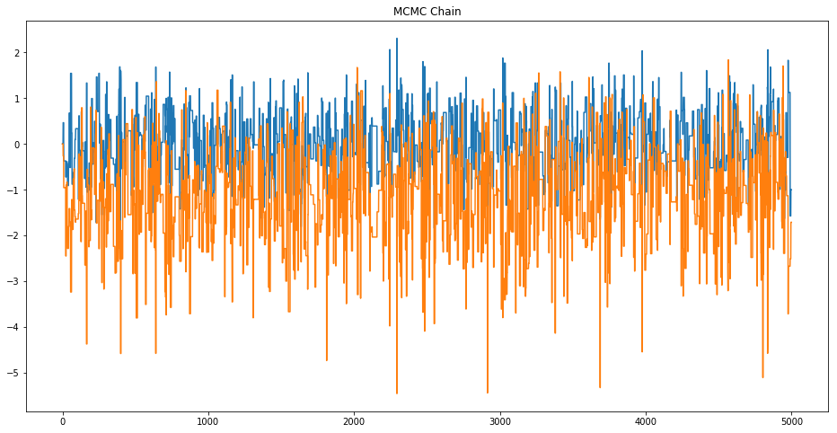
# TODO: Plot the MCMC chain.  Does it look like white noise?  Should it?

plt.figure(figsize=(16,8))

plt.plot(mcmcSamps[0,:])
plt.plot(mcmcSamps[1,:])

plt.title('MCMC Chain')
plt.show()

png

Importance Sampling

propMu = np.array([0,-4])
propCov = np.array([ [4, 0],
                     [0, 20]])

isProp = mm.Gaussian(propMu, propCov)

# TODO: Estimate the Banana density mean using an importance sampler

isSamps   = np.zeros((paramDim, numSamps))
isWeights = np.zeros((numSamps))

for i in range(numSamps):
    isSamps[:,i] = isProp.Sample()
    isWeights[i] = np.exp( tgtDens.Evaluate([isSamps[:,i]])[0] - isProp.LogDensity(isSamps[:,i]) )

plt.figure(figsize=(8,8))
plt.scatter(isSamps[0,:], isSamps[1,:], c=isWeights, alpha=0.5)
plt.title('Importance Sampling Points')
plt.show()

png

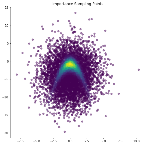
isMean = np.dot(isSamps, isWeights) / np.sum(isWeights)
print('Importance Sampling mean = ', isMean)

Importance Sampling mean =  [ 0.04996654 -1.99683488]

Inverse Problems: Systematic Integration of Data with Models under Uncertainty

2018 Gene Golub SIAM Summer School
June 17-30, 2018
Breckenridge, Colorado, USA

Introduction to Sampling Methods

Goals

Problem Description

Background: Simple Random number generation

Continuous Random Variables

Integer Random Variables

The MUQ `ModPiece` class

Derivatives in the `ModPiece` class

Sampling via Nonlinear Transformations

The WorkGraph class

Rejection Sampling

Markov Chain Monte Carlo Sampling

Importance Sampling

Inverse Problems: Systematic Integration of Data with Models under Uncertainty

2018 Gene Golub SIAM Summer School June 17-30, 2018 Breckenridge, Colorado, USA

Introduction to Sampling Methods

Goals

Problem Description

Background: Simple Random number generation

Continuous Random Variables

Integer Random Variables

The MUQ ModPiece class

Derivatives in the ModPiece class

Sampling via Nonlinear Transformations

The WorkGraph class

Rejection Sampling

Markov Chain Monte Carlo Sampling

Importance Sampling

2018 Gene Golub SIAM Summer School
June 17-30, 2018
Breckenridge, Colorado, USA

The MUQ `ModPiece` class

Derivatives in the `ModPiece` class