Bayesian Linear Regression
This lab is focused on Bayesian linear regression. Our goal is to estimate a function $f(x) : \mathbb{R}\rightarrow\mathbb{R}$ given $N$ observations ${(x_1,f(x_1)),\ldots, (x_N,f(x_N))}$.
Assume an approximation $\tilde{f}(x)$ of the form The regression problem is to characterize the coefficients $m=[m_0,\ldots,m_P]$, which we will do in a Bayesian setting.
Goals:
By the end of this lab, you will be able to
- Derive the posterior distribution for linear-Gaussian problems.
- Characterize prior and posterior predictive distributions.
Formulation:
Let $y$ denote the “observable” random variable denoting the models outputs and let $\bar{y}$ be a vector in $\mathbb{R}^N$ denoting the specific observations $f(x_1), \ldots, f(x_N)$. Our goal is to characterize the distribution of $m$ given $y=\bar{y}$. Bayes’ rule gives The two major components of this density are the prior density over the coefficeints $p(m)$ and the likelihood function $p(y|m)$. The prior represents should contain any information we might have before obtaining the observation $\bar{y}$. The likelihood function $p(y | m)$ defines a statistical model for the data.
For the prior distribution, we choose a Gaussian prior with a large variance. In particular, with $\sigma_m^2 = 100$.
Question: Do you think this is a valid prior? What if we knew $\frac{df}{dx}>0$? What would change?
To form the likelihood function, we need to relate the expansion coefficients $m$ with the observable random variable $y$. To do this, consider the Vandermonde matrix Using $V$, a common choice is to assume $y$ is given by where $\epsilon \sim N(0,\Sigma_y)$ is a zero mean random variable with covariance $\Sigma_y$. The additive error $\epsilon$ is often called the observation noise. Here, we will further assume that $\Sigma_y = \sigma_y^2 I$.
Question: Is this a reasonable model of $y$? What if the noise was multiplicative?
With this additive error, the likelihood function takes the form
Useful Identities
Let $\theta$ denote an arbitrary Gaussian random variable with mean $\mu_\theta$ and covariance $\Sigma_\theta$, Then, for a matrix $A$, Let $\eta = A\theta + e$, where $e\sim N(0,\Sigma_e)$, then the posterior $p(\theta | \eta)$ is given by where and
These notes by Sam Roweis also provide some useful identities.
Useful software references
Imports
import sys
sys.path.insert(0,'/home/fenics/Installations/MUQ_INSTALL/lib')

import numpy as np
import matplotlib.pyplot as plt

from PlotUtilities import PlotGaussianPDF
Generate Synthetic Observations
def TrueFunc(x):
    return np.sin(4.5*x)
numObs = 20
trueNoiseStd = 2e-2
obsLocs = np.linspace(0,1,numObs)

obsData = TrueFunc(obsLocs) + trueNoiseStd*np.random.randn(numObs)
numPlot = 100

plotx = np.linspace(-0.1, 1.1, numPlot)

plt.figure(figsize=(12,6))
plt.plot(plotx, TrueFunc(plotx),label='True Function')
plt.plot(obsLocs,obsData,'.', markersize=15, label = 'Observations')

plt.ylim([-1.2,1.2])
plt.legend(fontsize=16)
<matplotlib.legend.Legend at 0x7f79e7d22d68>
Form the prior
polyOrder = 4

priorMean = np.zeros(polyOrder+1)
priorCov = (10*10)*np.eye(polyOrder+1)
PlotGaussianPDF(priorMean,priorCov)
Prior predictive
predV = np.ones((numPlot,polyOrder+1))
for p in range(1,polyOrder+1):
    predV[:,p] = np.power(plotx, p)

predMean = np.dot(predV, priorMean)
predCov = np.dot(predV, np.dot(priorCov, predV.T))

predStd = np.sqrt(np.diag(predCov))
plt.figure(figsize=(12,6))

plt.fill_between(plotx, predMean-2.0*predStd, predMean+2.0*predStd, alpha=0.5, label='Predictive $\mu\pm2\sigma$')
plt.plot(plotx, TrueFunc(plotx), 'k', linewidth=3, label='True Function')
plt.plot(plotx, predMean, linewidth=3, label='Predictive $\mu$')
plt.plot(obsLocs,obsData,'.', markersize=15, label = 'Obs.')

plt.legend(bbox_to_anchor=(0., 1.02, 1., .102), loc=3, ncol=4, mode="expand", borderaxespad=0., fontsize=16)
plt.xlabel('Location $x$')
plt.ylabel('Load $m$')
plt.show()
Form the polynomial model
V = np.ones((numObs,polyOrder+1))
for p in range(1,polyOrder+1):
    V[:,p] = np.power(obsLocs, p)
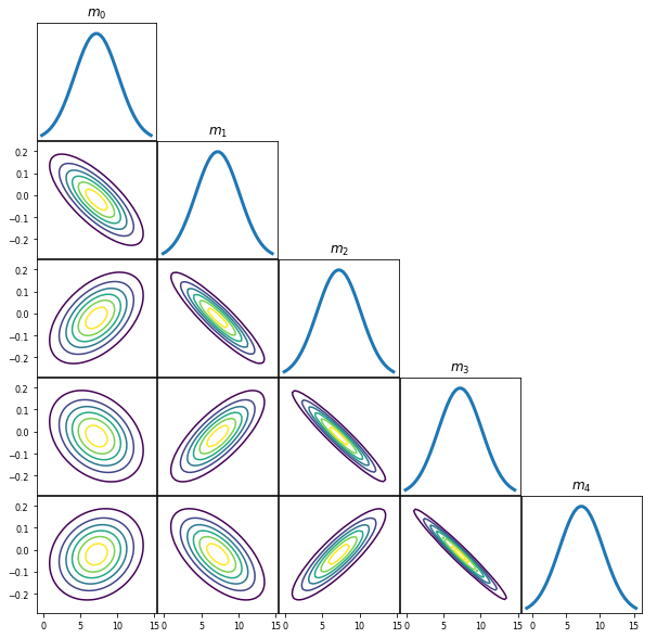
Compute the posterior distribution
modelNoiseStd = 1.0*trueNoiseStd
noiseCov = modelNoiseStd * np.eye(numObs)

Vsigma = np.dot(V,priorCov)
predCov = np.dot(Vsigma, V.T) + noiseCov

postCov = priorCov - np.dot(Vsigma.T, np.linalg.solve(predCov, Vsigma))
postMean = priorMean + np.dot(Vsigma.T, np.linalg.solve(predCov, obsData))
PlotGaussianPDF(postMean,postCov)

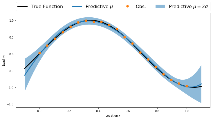
Posterior Predictive
predMean = np.dot(predV, postMean)
predCov = np.dot(predV, np.dot(postCov, predV.T))

predStd = np.sqrt(np.diag(predCov))
plt.figure(figsize=(12,6))

plt.fill_between(plotx, predMean-2.0*predStd, predMean+2.0*predStd, alpha=0.5, label='Predictive $\mu\pm2\sigma$')
plt.plot(plotx, TrueFunc(plotx), 'k', linewidth=3, label='True Function')
plt.plot(plotx, predMean, linewidth=3, label='Predictive $\mu$')
plt.plot(obsLocs,obsData,'.', markersize=15, label = 'Obs.')

plt.legend(bbox_to_anchor=(0., 1.02, 1., .102), loc=3, ncol=4, mode="expand", borderaxespad=0., fontsize=16)
plt.xlabel('Location $x$')
plt.ylabel('Load $m$')
plt.show()
Repeat with MUQ
import pymuqModeling as mm
Set up prior
priorMean = np.zeros(polyOrder+1)
priorCov = (10*10)*np.eye(polyOrder+1)

prior = mm.Gaussian(priorMean, priorCov)
PlotGaussianPDF(prior.GetMean(), prior.GetCovariance())

Compute posterior
post = prior.Condition(V, obsData, noiseCov)

PlotGaussianPDF(post.GetMean(),post.GetCovariance())
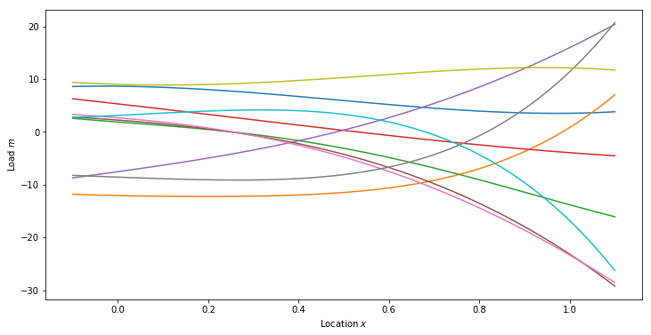
Prior Predictive Samples
numSamps = 10

priorSamps = np.zeros((priorMean.shape[0], numSamps))
for i in range(numSamps):
    priorSamps[:,i] = prior.Sample()

priorPredSamps = np.dot(predV, priorSamps)

plt.figure(figsize=(12,6))
for i in range(numSamps):
    plt.plot(plotx, priorPredSamps[:,i])

plt.xlabel('Location $x$')
plt.ylabel('Load $m$')
plt.show()
Posterior Predictive Samples
numSamps = 10

postSamps = np.zeros((priorMean.shape[0], numSamps))
for i in range(numSamps):
    postSamps[:,i] = post.Sample()

postPredSamps = np.dot(predV, postSamps)

plt.figure(figsize=(12,6))
for i in range(numSamps):
    plt.plot(plotx, postPredSamps[:,i])

plt.xlabel('Location $x$')
plt.ylabel('Load $m$')
plt.show()